
The best way to learn R is to use it! With data! This page walks you through some example data analyses using environmental data (and assumes you have worked through the StartR page first). The steps through the analyses are shown in the first section, using text and videos, for R only. Once all the analyses have been performed in R, we’ll see in the second section how RStudio would be used to the same end.
It’s important that you try the process in R first, so that you can understand how R itself works and because learning code is best done by typing the code yourself (not copy&paste). As you develop your understand you can switch to use RStudio for all your analyses.
The data for this exercise are available to King’s students, either through a relevant KEATS page (e.g. Methods for Environmental Research) or can be requested by email (using your @kcl.ac.uk address) from James.
1. Data Analysis with R
1.1 Data Familiarisation
Let’s move on now to see how we can use R to actually do some data analyses. We will be investigating river levels of the River Frome, Dorset. The data we will be using are from a pressure transducer placed at Frampton on the River Frome, which recorded river levels from May 2003 to April 2005 (data used in the practical are from Moggridge and Goodson, 2005) and is ‘site B’ in Gurnell et al. (2006). Pressure transducers (PTs) measure the pressure produced by a column of water above a sensing element. As water exerts more pressure than air, the higher the pressure recorded by the PT, the higher the water level. These readings were taken every 15 minutes for the duration of the study and recorded in a data logger. In addition to Gurnell et al. (2006), who conducted their research for both of their study sites near Dorchester, you will find Cotton et al. (2006) to be a useful reference, as one of their study sites was also near Dorchester.
1.2 Loading and Viewing Data
Because R is a statistical environment it does not store data permanently. To use existing data, it must be stored in external files on a hard disk that are loaded into memory in R. Once in memory, work can be done and the resulting data output (to memory, but later this can be written to hard disk in a file).
One of the best ways to store data on a hard disk for use in R is a file format known as Comma Separated Values (csv). These files are simply text files in which each value in the data table is separated by a comma. Because of its simplicity, this file format can be opened in many software packages, including Excel and text editors (and R, of course).
Data from (Moggridge and Goodson, 2005) are provided for use in R in two files (listed below, available on KEATS):
- LoggerData.csv – the data from the logger
- WaterLevelData.csv – the calibration of the recorded pressure and the corresponding relative water level of the river
Metadata (data about the data) for these data are shown in Table 1.
Table 1. Metadata for River Frome data
| File | Field | Units | Description |
| LoggerData.csv | |||
| ID | NA | identification number of the logger | |
| Year | year | year the data was recorded in | |
| Day | Julian Days | date of the record, in Julian Days (which record dates in a calendar year 1-365) | |
| Time | time | time of the recording, in 24 hour format | |
| Pressure | mV | the pressure recording | |
| Battery | V | battery power remaining (important if there are any anomalies in the data due to battery failure). | |
| InTemp | celcius | temperature inside the logger container | |
| ExtTemp | celcius | temperature of the surrounding air | |
| WaterLevelData.csv | |||
| DateTime | NA | date and time of recording | |
| Pressure | mV | the pressure recording | |
| WaterLevel | meters | water level in metres above an arbitrary datum |
The easiest way to view and familiarise yourself with these data (as you always should) is to open them in Excel or a text editor (like notepad or EditPad). However, if we are to use these data in R we must first read them into memory.
For this exercise we are going to read csv files into R. To make things simple this file should contain only the data with the headers for columns. To read in the file, first you will need to download the csv files to a ‘working directory’ (simply the folder where you will save the data to work with now). Once the files are downloaded and saved you will need to let R know what the location of your working directory is on the computer’s hard disk. To do this, use the ‘set working directory’ command setwd(). For example, if your data are saved in a folder called Practical1 in your My Documents folder on the N drive you would set the working directory at the command prompt using something like:
setwd(‘N:/My Documents/Practical1’)
Above, we have provided ‘N:/My Documents/Practical1’ as an argument (which contains a ‘path’ – as shown for Mac here). To check you have set the working directory correctly, enter the following command:
getwd()
To read the csv data into memory in R we use the read.csv() function. As we have specified the current working directory now we can call the read.csv() function with the filename alone. We also need to specify that the first row of the file is a header for column names [to see all the options for the read.csv() function use help(“read.csv”)]:
loggerDat <- read.csv("LoggerData.csv", header = T)
With this command we are assigning the data from file to an object named loggerDat. The header = T argument is telling R that the first row of the input file contains the names of the columns. To check the data have loaded properly we can view the first few lines of the data file using the head() function:
head(loggerDat)
If your data have been loaded properly you should see something similar to Figure 1. You can also see a summary of the data you have loaded using the summary() function. Follow the same procedure as above to load “WaterLevelData.csv” to an object named waterDat.

Figure 1. Data logger data in R
A video showing the above steps:
Using the water level data, we can quantify the relationship between pressure and water levels and apply this relationship to the remainder of the logger data, to obtain a continuous estimate of water level. We will do this using a technique called linear regression, which we will cover in more detail later on in the module. First we will create a scatterplot to check what the data look like so that we can better visualise what we are doing.
1.3 Creating a Scatterplot
To create a scatterplot of data in R, we can use the plot() function. This function requires that we specify two vectors (columns) of data, one for the x-axis (pressure) and one for the y-axis (water level) as follows:
plot(waterDat$Pressure, waterDat$WaterLevel)
The $ symbol specifies which field (column) in the data is being referred to; so waterDat$Pressure is the Pressure field (column) of the waterDat data frame (table) . This should produce a plot in another window within R. To format the plot to make it look nicer we can add more arguments to the plot() function as follows:
plot(waterDat$Pressure, waterDat$WaterLevel, xlim = c(0, 0.6), xlab = "Pressure (mV)", ylim = c(99.0, 99.4), ylab = "Water Level (m, above an arbitrary level)", main = "River Frome, Dorset")
Each of the additional arguments works as follows:
- xlim: sets the limits (min, max) of the x-axis
- ylim: sets the limits (min, max) of the x-axis
- ylab: the label to be added to the y-axis
- main: the main title of the plot
There are many resources online on how to format plots in R. The package ggplot2 is fast becoming the best way to plot data using R.
A video showing the above steps:
1.4 Simple Linear Regression
From your plot you should see a clear pattern in the data. You can now perform a simple linear regression on these data, which will create a line of best fit. We can then use the equation of this line to predict the water levels from a known pressure.
To fit a regression in R we use the lm() function (lm for ‘linear model’), as follows:
fit <- lm(WaterLevel ~ Pressure, data = WaterDat)
This has fit the regression and created an lm object named fit. To see information about the fitted regression model we can use the summary() function:
summary(fit)
To get the goodness of fit value (r2) for the regression model we have fitted, we use:
summary(fit)$r.squared
Again we see the $ symbol allows us to access elements from within an object (in this case the r.squared value from the result of the summary(fit) command). The r2 value gives an indication of the ‘goodness of fit’ and ranges from –1 to 1 (with 1 being a perfect linear relationship, 0 no relationship, and –1 a perfect inverse linear relationship of the y value with x). Does your regression line have a good fit?
We can now use the lm object (which we have named fit) to plot a regression line on our plot. We do this with the abline() function, passing the fitted regression model as the argument:
abline(fit)
You should now see the regression line added to the plot, similar to that shown in Figure 2.
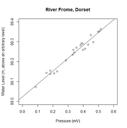
Figure 2. Scatter plot with regression line from R
A video showing the above steps:
1.5 Predicting from a model
The equation of the simple linear regression you have created allows you to predict h (i.e., water levels) from a known value of p (i.e., mV). To calculate the River Frome water level from the pressure data collected we can now use our fitted regression model with the predict.lm() function:
PredictedWL <- predict.lm(fit, loggerDat)
Here we have assigned the estimated water level data to an object named PredictedWL. This object is a vector (column) of 66990 values (one for each pressure value in the logger data). To check the size of the vector, we can use the length() function:
length(PredictedWL)
As this is a very long vector we probably don’t want to inspect every value, but we should at least inspect some to check the values are on the order we expect. To do this we can use the head() function to print the first few values of the vector:
head(PredictedWL)
Do these values look appropriate?
To continue to use these data we will attach the PredictedWL vector to the original data using the cbind() (column bind) function:
loggerDat <- cbind(loggerDat, PredictedWL)
This is the equivalent in Excel of copying the column of predicted values and pasting them into a column next to the other values in the logger data such that they compose a single data matrix (i.e. table of values). Check this worked properly by using the head() function on the loggerDat object.
Finally, this new data matrix (table) can be written out to a new file using the write.csv() function:
write.csv(loggerDat, "conversion2.csv", row.names = F)
You can read about the arguments for the write.csv() function (e.g. to help understand what row.names = F does) by entering help(“write.csv”) at the command prompt. The file should have been written to the same directory (folder) where your original data were saved on your computer. Plots can be written to an image or pdf format file.
A video showing the above steps:
1.6 Aggregating Data
As there are very many data from the Logger (collected every 15 minutes) we can create daily summaries of the water level to reduce the number of values we plot in a time-series. To do this, we can use the aggregate() function. We first remove the ID column of the data (which is redundant in this case):
loggerDat <- loggerDat[,2:9]
If you can, try to think about what this line of code is doing; it taking a subset of columns (numbered 2-9) in the ‘original’ data object and assigned it to a ‘new’ object with the same name (i.e. effectively over-writing the original object). To see the difference, use the head() function and compare to the csv file you wrote to disk in the previous section.
Now we can aggregate our data by year and day, calculating the mean for each variable in our data, as follows:
aggLoggerDat <- aggregate(loggerDat, by = list(loggerDat$Year, loggerDat$Day), mean)
These aggregated data are initially ordered by Day and then Year, but we want them order by Year then Day. To do this we use the order() function (this is similar to sorting in Excel):
aggLoggerDat <- aggLoggerDat[order(aggLoggerDat$Year, aggLoggerDat$Day),]
Quickly remove the two columns created by order function:
aggLoggerDat <- aggLoggerDat[,3:10]
These new data can be written to file as before:
write.csv(aggLoggerDat, "aggLoggerdata.csv", row.names = F)
A video showing the above steps:
1.7 Plotting a Time-Series
A line plot of the predicted water level data through time is easily created in R using the plot() function, specifying a line plot:
plot(aggLoggerDat$PredictedWL, type = "l")
To format the plot more nicely, we can call the plot() function again but with some additional arguments:
plot(aggLoggerDat$PredictedWL, type = "l", xlab = "day", ylab = "Predicted Water Level (m)")
If we wanted to plot only a subset of the data we could use the subset() function to create a new data.frame (table) which could then be plotted:
aggLoggerDat.2003 <- subset (aggLoggerDat, Year == 2003)
A video showing the above steps:
1.8 Saving Images to File
To write this new plot to an image file that is saved on the disk we need to use a sequence of three commands (in the right order!). Enter each line below, pressing enter between each:
jpeg("aggLogger2003.jpg")
plot(aggLoggerDat.2003$Day, aggLoggerDat.2003$WaterLevel, type = "l", xlab = "day", xlim = c(0,365), ylab = "Predicted Water Level (m)")
dev.off()
As above, this file should have been written to the same directory (folder) where your original data were saved on your computer. You can now paste this image into a word document (for example).
A video showing the above steps:
2. Analysis with Scripts
All the R commands in the data analysis section above can be found in the FromeAnalysis.r ‘script’. A script is a series of commands saved in a text file that can be saved for later use. Note that usually R script files usually have a suffix .r (as in FromeAnalysis.r) rather than the more standard .txt for text files. Your computer may not know what to do with a .r file if you double-click on it, but if you open the file from R or RStudio you’ll be fine.
The great thing about scripts is that once they have been saved they can be re-run at a later time. This means you can close your script, re-open it (from the file menu) and run it again anytime you want. Using scripts is a very efficient way of running analyses and provides a means of recording and replicating your analyses (important for the Scientific Method!).
The text file containing the script can be created and run in the script editor that comes with the standard installation of R or in a stand-alone text-editor (such as notepad). However, other software environments such as RStudio have been created for use with R to facilitate the use of scripts. You should already be somewhat familiar with how to use script in RStudio from the video on the StartR page.
However, to give you a little more guidance on how to use RStudio, the video below shows all the Frome River analysis from above performed in RStudio (without typing all the code out!). Download the FromeAnalysis.r script and follow the video to make sure you understand what is going on (make sure you have saved the data from KEATS in the appropriate directory!).
Reading the ‘comments‘ in the script file should also help. Comments in R are indicated by # – anything in a line after this symbol are ignored by R. Comments are both important for sharing code with others and to remind your future yourself what you are aiming to do with your code!
Before you go… Packages
Hopefully these materials were useful to get you started with R and RStudio, but there is plenty more to learn because ‘packages’ for R are continually being created which provide a huge range of functionality. Packages are collections of functions (commands) that people have written to that they are readily available for others to use. Some packages are pre-installed when you install R on your computer, but for many others you will need to download and install them before you can use them. Installation of packages can be done either in R itself, or in RStudio using the packages tab:
Most packages you will need for modules at King’s should be installed on King’s computers. However, if a package you want to use is not already installed you should be able to install it to a a personal library directory in your home folder and it should then be available when you log into another machine.
Once a package is installed you then need to load it so that you can use it. In RStudio, you can do this by checking the box next to the package name in the package tab. But usually more useful (e.g., so you don’t forget if you ever use your script again later) is to load it using code:
library("ggplot2")
The code above would load the ggplot2 library (assuming it had been installed on the computer on which you are using). Now you have access to all the wonderful graphical functionality ggplot2 provides!
The final question you may have is how do you know which packages are useful for what you want to do? One way is to search the lists of packages on CRAN. The other is… google it!
More LeaRning Resources
If you’re hungry to leaRn more right now, checkout these great resources:
- Code School
- Cyclismo Tutorial
- Tutorials Point
- Huge list of R tutorials
- Swirl (tutorials within R)
References Cited
Cotton, J.A., Wharton, G., Bass, J.A.B., Heppell, C.M. and Wotton, R.S. (2006) The effects of seasonal changes to in-stream vegetation cover on patterns of low and accumulation of sediment. Geomorphology, 77, 320-334.
Gurnell, A.M., Van Oosterhout, M.P., Vlieger, B.D. and Goodson, J.M. (2006) Reach-scale interactions between aquatic plants and physical habitat: River Frome, Dorset. River Research and Applications, 22, 667-680.
Moggridge, H. and Goodson, J. (2005) River Frome Electronic Data. Collected as part of NERC research grant NER/T/S/2001/00930 (LOCAR programme).
The content and structure of this teaching project itself is licensed under the Creative Commons Attribution-NonCommercial-ShareAlike 4.0 license, and the contributing source code is licensed under The MIT License.
