
This page is intended to get you started on the path to using R with RStudio for your quantitative data analysis.First, we offer some guidance on how to install R and RStudio on your own computer. Then we provide an overview of R and RStudio and some first steps of use. Once you’ve gone through these basics you should moved on to try the example of some data analysis using R and RStudio we’ve put together.

R is a statistical and data analysis language that enables a wide range functions for quantitative analysis and data visualization. Executing these functions through code rather than using a mouse with a Graphical User Interface (GUI) enables reproducible analyses – so you can repeat the analyses later, whether on the same data or new – and the automation of tasks – so that you can do the same thing over and over many times very quickly.

RStudio is an Integrated Development Environment (IDE) that enables more efficient and flexible use of R. Although R is very powerful and is essentially code-based, RStudio provides a wrapper around that code base that makes it easier to do things like save ‘scripts’ of code to use later, view data that has been loaded into memory, export graphs output from your code, and install R packages (libraries of functions).
Installing R and RStudio
Note that R and RStudio are installed and available on all King’s Campus computers, so you will only need to follow the instructions in this section if you wish to use R or RStudio on a personal computer (otherwise, skip on to the overview section).
Installing R
R is open source and freely available for installation on personal machines. There are many resources online explaining the installation process for R, including useful videos for Windows and Mac on YouTube. NB: keep when reading any other resources that installing an ‘R package’ is not the same as installing the R software itself (we’ll look at R packages later).
Essentially, the steps to install R on your personal computer are:
- Go to the Comprehensive R Archive Network (CRAN) website and click on the link to a mirror (server) geographically close to your location: https://cran.r-project.org/mirrors.html. For example, if you are in London you might pick the Imperial mirror.
- From the mirror page, in the Download and Install R section click the link for your operating system. For Windows for example, click the Download R for Windows link.
- The subsequent pages will look different depending on your operating system:
- For Windows: click on either base or install R for the first time link (even if you have previously installed R) and then from the subsequent page click the link at the very top that will say Download R 4.1.1 for Windows (or similar). The installer will either immediately begin to download or you will be prompted to save the file.
- For Mac: click on the link for the first package file in the list of files. This link will be R-4.1.1.pkg or similar. The package should automatically download to your computer.
- With the relevant installer downloaded (on both operating systems), launch the installer (e.g. on Windows double click the icon your downloads folder).
- Once the installer has launched simply follow the instructions! (Install for all users if you are prompted and generally all the default options will work well).
At this point you might check that R has installed correctly by trying to launch it. For example, in Windows you will usually have a link in the Start Menu. On Mac, the R icon should now appear in your applications folder. If you have successfully installed a new window should appear with text that looks something like Figure 1.
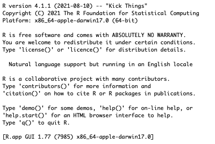
Figure 1. The R startup text. If you see text that looks something like this appear in a window, you have successfully installed and launched R!
Installing RStudio
RStudio is open source and freely available for individual use. Remember, R and RStudio are installed and available on all King’s Campus computers, so you will only need to follow the instructions in this section if you wish to use RStudio on a personal computer (otherwise, skip on the overview section).
An important point to highlight right from the start is that you should only install RStudio after you have installed R, so if you haven’t done that yet stop here and install R. The installation process for RStudio is pretty similar to that for R, but with fewer webpages to click through:
- At the RStudio Downloads page, scroll to the bottom to find the section named Installers for Supported Platforms and click the appropriate link for your operating system. Make sure that you are getting the installation file for RStudio Desktop (not RStudio Server).
- The next step varies for Windows and Mac:
- For Windows you will need to find the installer you just downloaded in your downloads folder and double-click to launch it. Follow the installation instructions from there. Watch a video on how to install for Windows here.
- For Mac, you need to copy the file downloaded into your Applications folder. RStudio should then be ready to launch. Watch a video on how to install for Mac here.
If installation of both R and RStudio has gone well, when you launch RStudio you should see a window like something like that shown in Figure 2 (if you only have three panes don’t worry as long as one of them contains the R startup text as in Figure 1).
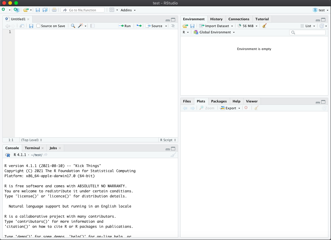
Figure 2. The RStudio window after successful installation of both R and RStudio. Note the R Startup Text from Figure 1 in the lower left pane of the window.
Overview of R and RStudio
As R is the workshorse here, and RStudio just a wrapper around it which offers some nice extras, we’ll start by looking at the basics of R itself before moving on to RStudio.
StartR
The first thing to know about R is that it is driven typing commands to tell the software what to do, rather than hunting and clicking through menus. This approach is more versatile than a GUI, and allow us to save commands in a ‘script’ to be executed all in one go, but it does take some getting used to if you are someone who rarely takes their hands off their mouse.
When you open up R, you should see something like shown in Figure 1 and the start of the video below. The command prompt in the console window is the red ‘greater than’ symbol (>). Commands are written at the prompt and hitting Enter tells R to execute the command.
At its most simple a command could be an equation like you would type into a calculator:
> 2 + 2
Try it in R now!
All the commands in the objects section below are shown in the video above – make sure you try the commands yourself in R (using the video to help if necessary) to ensure you understand what is being done.
Objects
More complicated commands may create ‘objects’ and assign values to them. For example, if we wanted to save the result of our equation above we could create an object and assign the result of the equation to it:
> answer <- 2 + 2
assigns the result of the equation to an object named answer. This result is now held in the computer’s memory. We can later view the result by calling the ‘print’ function, passing the name of the object we want as an ‘argument’ (more on arguments below):
> print(answer)
Another way we could have done the addition equation was by using the sum function:
> answer <- sum(2,3)
If you print the answer object now you will see it has been updated (i.e. overwritten) with the new result. Try this now.
We can also create new objects using existing objects:
> another.answer <- sum(answer,5)
Try this yourself. What do you get when you print the result of another.answer?
If a command gets so long that it breaks onto the next line, or if you hit Enter without completing a command, R will prompt you on the next line with a plus sign (+). This means there is more to add to the command before it can be executed. This often happens, for example, when you don’t close a parenthesis (e.g. see from 1min 13 secs in the video above).
In that example, the closing (right) parenthesis was not typed before enter was hit (to print another.answer). All that needs to be done to fix this is to provide the closing parenthesis (by typing ) and then hitting Enter (also shown in the video).
You must also ensure you spell all objects, functions, etc. correctly (with correct case) otherwise R will not know what to do and give an error message (shown at 1min 27secs in the video).
Functions
Functions are built-in bits of code that mean we can quickly ask R to do several sets of commands all-in-one. For example, say we have a series of numbers that represent the diameters of individual trees you have measured, and we want R to calculate the mean (i.e. average) tree diameter for us. Let’s also say we’ve saved this series of numbers in R as an object named TreeDiameters. In this case, R can quickly do the calculation for us via the mean function:
> mean(x = TreeDiameters)
Note here that mean is the function name, x is the argument and TreeDiameters is the value passed to the argument. The above is a specific example of the general form needed to execute an R function:
> FunctionName(argument1 = a, argument2 = b, ...)
where FunctionName is the name of the function you wish to execute, argument1 and argument2 are the names of arguments that can be passed to the function, a and b are values that the arguments will be given (these might be numbers or text), and … are other arguments or options that you may want to pass to the function (some functions can take many, many arguments). Often the names of arguments can be dropped and you can simply provide the value [a and b in this example: FunctionName (a,b) or x in the example above: mean(TreeDiameters)].
But how did I know that there was a function called mean and that x was the first argument needed? Well that knowledge will come to you through time, by reading and googling. Note that the standard R help manuals can be a little abstruse at times, but that there are many, many, many other resources online that will be useful to draw on when learning R. And there are some great tutorials online, some of which are interactive. And don’t be afraid to google something – the chance is that if you have a question, someone else has had the same one before you!
For example, from the help page for the mean function (found via google) we can see that one of the optional … arguments is na.rm which we could include like this:
> mean(x = TreeDiameters, na.rm = T)
In this case the optional argument, na.rm = T tells R to remove any missing values from the data series before calculating the mean.
Note that the parentheses are mandatory for a function, even if there are no arguments or options given. For example, the following is the command for the ls function that lists all the objects currently loaded in R’s memory:
> ls()
If the name of a function is typed without parentheses, R will print out the programming code for the function. This can be quite surprising but need not be scary – you haven’t broken anything! Just try again, this time with the parentheses.
Computers are Stupid!
The examples above highlight several important points to remember when typing commands at the prompt (or when writing a script – see below) to make sure things work properly:
- R is case-sensitive; Mean(TreeDiameters) is not the same as mean(TreeDiameters) or mean(treediameters)
- As the line break example in the video shows, commands must be correctly formatted: commas must be in the right place, parentheses must be closed, etc.
- You must get the spelling of commands, arguments, etc. correct!
It may be frustrating initially, but you must remember that computers only do what you tell them and ultimately it is up to you, the user, to get your commands right!
Basics in RStudio
Now that we’ve seen the basics of R, let’s see how we might do the same in RStudio. But now we’ll also look how RStudio can help us save the commands for later, how we can quickly view data and objects stored in memory, get ready access to help pages, and view and export plots. RStudio have provided a nice overview themselves in the video below.
As shown in Figure 2 and the video, RStudio usually has four panes:
- the lower left is the ‘console pane’
- the upper left is the ‘source pane’
- the upper right is the ‘workspace’ pane
- the lower right is the ‘plots-help’ pane
[If you can’t see the source pane and have a very long console pane, you may need to open a new script: go to File menu -> New File -> R Script. Shown in the video below.]
The console pane is essentially exactly the same as the console window we see in R itself; we could type exactly the same commands as we did above in this pane with the same effect. This embedded view of R within RStudio is one reason we can think of RStudio as a wrapper around R.
The source pane allows us to view text files of saved commands (known as ‘scripts’) and to run these commands without needing to type them again into the console pane. Using scripts can save us time and allow us to repeat and reproduce our analyses in future – very handy!
The workspace pane has two tabs at the top (by default), allowing us to switch between two views. The ‘environment’ view allows us to see all objects loaded into memory; some objects, like DataFrames, will display in the source pane when clicked on (others will not). The ‘history’ view allows us to see a list of commands recently executed.
The plots-help pane has multiple tabs (more than just three), allowing even more different views. The views to consider here are the help view, which allows quick access to the R help manual pages (with search function), and the plots view, which contains all plots (use arrows to move back and forth) and a button to enable quick export to an image file (e.g. for use in a report or presentation).
The video below shows use of all of these panes to analyse tree diameter data with a script that uses many of the commands highlighted above. The data used in the video are modified from the Harvard Forest Data Archive and can be downloaded here (right/ctrl click that link and then ‘save as’, otherwise a left-click should download the file, even if a 404 broken link is indicated). The script file used in the video can be downloaded here. See if you can use these two files to repeat the simple analyses shown in the video.
Hopefully the overview and videos above have given you an idea about how to get started using RStudio, but there’s lots more to learn. Examples of resources available include:
- books like Robin Lovelace’s Geocomputation with R [online version]
- websites like the RStudio documentation pages
- YouTube videos like this one by R Tutorials (also great if you’re still confused about the difference between R and RStudio!)
But the best way for you to really learn R and RStudio is to use it with data! If you don’t need a break to digest everything above, move on to try this example data analysis.
The content and structure of this teaching project itself is licensed under the Creative Commons Attribution-NonCommercial-ShareAlike 4.0 license, and the contributing source code is licensed under The MIT License.
